ConviviaR Tools: Zodiac Charts

Aleksei Lutai

Why the parliaments? Or it could be “How dare you to look at our Parliament”? My thinking is that if there is any zodiacal influence (which I am not sure myself), I would expect it to be manifested to much higher extent amongst the politicians - as their work requires a very specific blend of moral, ethical, and personal traits. The politicians are also public persons, so it is not a problem to obtain their birth dates.

This is very much not a fundamental research with probabilities and null-hypotheses, there will be no solid proofs or conclusions. It’s just an exercise on using ggplot, wikidata, and the fonts.

Since I know too little about astrology, I have to plead my ignorance for possible incorrect use of the terms and not going deeper. Wikipedia, I guess, could be a starting point for you to become acquainted with the basics:

In the text below I use a term “west zodiac” for the astrological signs like Libra or Virgo, and the terms “east zodiac” or “chinese zodiac” for the years of Dragon, Tiger, etc. Please do not take it as offence, if you think that the chosen names are kind of inappropriate.

Notes on Code

There are few things that can help you to understand and adopt this script:

during the session I save the fonts and the downloaded data into a folder encoded in the variable dir_data, the charts – into a folder set as dir_charts. The code in the other chunks will be using those variables for saving and loading, so if you decide to use this routine, set the folder names according to your data management plan.

Show code

dir0 <- "D://tmp_data/"
if(!dir.exists(dir0)){ dir.create(dir0) }

dir_data <- paste0(dir0, "data/")
if(!dir.exists(dir_data)){ dir.create(dir_data) }

dir_charts <- paste0(getwd(), "/images/")
if(!dir.exists(dir_charts)){ dir.create(dir_charts) }

in the chunks where something is getting downloaded, I usually check if the destination file already exists to avoid double saving and speed up the script running.
In some cases I will have to parse the dates written as 01 Jan 2024 or 15 July 1918. If your regional setting are not english (like mine), most likely you will have to set the time locale as english (see below).

Show code

Sys.setlocale("LC_TIME", "english")

[1] "English_United States.1252"

Fonts

In this project I am using 2 fonts with the zodiac glyphs and some other fonts for styling. The showtext package have a nice option to load the google fonts from internet (see vignette), but I am cautious about making my scripts too much dependent on the internet’s availability. That’s why in the script below the fonts are loaded from a local storage of my favourite fonts, referred as local_font_folder.

If you decide to use special fonts, you will have to set the correct paths to the font files (or you can try to use sysfonts::font_add_google()).

Essential TTF Fonts:

Chinese Zodiac (I could not find its creator). The font can be downloaded from many web sites like onlinewebfonts.com.
SL Zodiac Stencils Font (download from FontSpace, created by Su Lucas.

I referred to these fonts as essential in a sense that you need to have these fonts at hand to draw zodiac charts. I downloaded them manually and saved into my local font storage as east_zodiac.ttf and west_zodiac.ttf.

Other Fonts

In this project I use for styling few other fonts, distributed with SIL Open Font License (OFL):

and

Font Awesome 6 for the icons.

The script below shows how to load the fonts.

Show code

showtext_auto()

sysfonts::font_add("zodiac", regular = paste0(local_font_folder, "/astro.ttf"))
sysfonts::font_add("ch_zodiac", regular = paste0(local_font_folder, "/chn_zodiac.ttf"))

font_add("RobotoC", regular = paste0(local_font_folder, "RobotoCondensed-Regular.ttf"))

font_add("Sofia", 
         regular = paste0(local_font_folder, "SofiaSansCondensed-SemiBold.ttf"),
         bold = paste0(local_font_folder, "SofiaSansCondensed-SemiBold.ttf"))

sysfonts::font_add("fa_solid",
                    regular = paste0(local_font_folder, "/fontawesome/otfs/Font Awesome 6 Free-Solid-900.otf"))

Styling (ggplot2 theme)

Show code

blankbg <- theme(axis.line = element_blank(),  
                 axis.text=element_blank(),
                 axis.ticks=element_blank(),  
                 axis.title = element_blank(),
                 plot.background=element_rect(fill = "#232323", colour = "#232323"), 
                 panel.background=element_rect(fill = "#232323", colour = "#232323"),  
                 panel.border = element_blank(),
                 panel.grid.minor=element_blank(), 
                 panel.grid.major = element_blank(),
                 plot.margin = unit(c(t=0.2,r=0.05,b=0.2,l=0.05), "cm"),
                 plot.title.position = "plot", 
                 plot.caption.position = "plot",
                 plot.title = element_text(size = 22, hjust = 0, 
                                           face = "bold", colour = "#ffffff", family = "Sofia"), 
                 plot.subtitle = element_text(hjust = 0, family = "RobotoC", vjust = 2,  
                                              colour = "#ffffff", face = "plain", size = rel(0.7)),
                 plot.caption = element_markdown(halign = 0, hjust = 0, 
                                                 size = rel(0.8),colour = "#827C82"))

showtext::showtext_opts(dpi = 192)

Extra Data

The fonts need to be correctly associated with the zodiac names and the preferred order. For this I create the small tables where the letters correspond to zodiac symbols (a letter against each zodiac sign corresponds to its graphical representations provided by the font).

The tables below are created with a tribble function, you may just copy/paste it into your script, and tinkle further as you wish (for example, change the order values to ensure that some particular sign opens a list).

Show code

west_symbols <- tibble::tribble(
  ~unicode, ~sign, ~order, ~letter, 
  "\u2652", "Aquarius",1, "k",
  "\u2653", "Pisces", 2, "l",
  "\u2648", "Aries", 3, "a",
  "\u2649", "Taurus", 4, "b", 
  "\u264A", "Gemini", 5, "c",
  "\u264B", "Cancer", 6, "d",
  "\u264C", "Leo", 7, "e",
  "\u264D", "Virgo", 8, "f",
  "\u264E", "Libra", 9, "g",
  "\u264F", "Scorpio",10, "h",
  "\u2650", "Sagittarius", 11, "i",
  "\u2651", "Capricorn", 12, "j"
) 
paged_table(west_symbols, options = list(rows.print = 6))

Show code

east_symbols <- tribble(
        ~sign, ~order, ~letter,
        "Rat", 1, "a",
        "Ox", 2, "b",
        "Tiger", 3, "c",
        "Rabbit", 4, "d",
        "Dragon", 5, "e",
        "Snake", 6, "f",
        "Horse", 7, "g",
        "Goat", 8, "h",
        "Monkey", 9, "i",
        "Rooster", 10, "j",
        "Dog", 11, "k",
        "Pig", 12,"l")
paged_table(east_symbols, options = list(rows.print = 6))

Western zodiac signs (Libra, Capricorn, etc) are easy to calculate, as the date ranges are the same for each year (i.e. Taurus period is always from 21.04 till 21.05). So it’s just 12 date ranges to be matched against to get a astrological sign for any birth date. I found a package DescTools providing a function named Zodiac. Its using is as simple as DescTools::Zodiac(birth_date, lang = “eng”), where birth_date is a date in POSIXlt format.

With Chinese zodiacs (Rat, Rooster, Dragon, etc) things are a bit more complicated, as the Chinese New Year date is not fixed. Yes, the years begin on different dates, you my check Wikipedia article Chinese calendar for additional details. I extracted the Chinese zodiac years from Wikipedia/En article named Chinese zodiac.

First, I use API call to get a list of sections for the article: https://en.wikipedia.org/w/api.php?action=parse&page=Chinese_zodiac&prop=sections. The section Years contains a Table with the Chinese zodiac years from 1924 till 2044, its index is 4.

Next, I use API call to obtain an html for the section 4, and extract the table data (see code in the chunk below).

Show code

ch_dates_file <- paste0(dir_data, "ch_dates.RDS")
if(!file.exists(ch_dates_file)){
  ch_dates <- "https://en.wikipedia.org/w/api.php?action=parse&page=Chinese_zodiac&section=4&prop=text&format=json" |>
    rvest::read_html(encoding = "utf8") |>
    rvest::html_table(trim = T) |> pluck(1) |>
    select(year1 = 2, year2 = 3, element = 4, heavenly_stem = 5, earthly_branch = 6, sign = 7) |>
    # first row does not contain the data, it originates from 2-level table header.
    filter(row_number()>1) |>
    pivot_longer(contains("year"), names_to = NULL, values_to = "year") |>
    separate(year, sep = "\\\\u2013", into = c("date_start", "date_end")) |>
    separate(element, sep = " ", into = c("element_ch", "element_en")) |>
    mutate(sign = str_replace(sign, "\\\\n", ""),
           across(contains("date"), ~as.Date(.x, "%B %d %Y"))) |>
    arrange(date_start) |> 
    left_join(ch_symbols)
  
   write_rds(ch_dates, ch_dates_file)
} else {
  ch_dates <- read_rds(ch_dates_file)
}

paged_table(ch_dates, options = list(rows.print = 6))

Now we are ready to collect the data with the birth dates.

Data

Wikipedia and Wikidata have versatile APIs to ease our collecting the birth dates of the selected parliaments. Below I use SPARQL queries to Wikidata in order to get the birth dates for a particular group of parliament members.

In some cases a number of parliament members were a bit different than it should be according to the corresponding Wikipedia articles. Some members may not be present or may not have a birth date in Wikidata. Or some persons may be inaccurately assigned to a chamber of parliament, being not an MP, but member of committee or something. I am not an expert in the electoral and mid-electoral lifecyles in the national parliaments, so I did not try to seek the causes. The data is provided as it is collected from Wikidata.

Members of the 9th European Parliament

Show code

eu_file <- paste0(dir_data, "eu_data.RDS")
if(!file.exists(eu_file)){
  eu <- query_wikidata('SELECT DISTINCT ?item ?dob WHERE {
                     ?item p:P39 ?pSt. ?pSt ps:P39 wd:Q27169; pq:P2937 wd:Q64038205. 
                     OPTIONAL {?item wdt:P569 ?dob.}}') |> 
    na.omit()
  write_rds(eu, eu_file, compress = "gz")
 } else {
   eu <- read_rds(eu_file)
  }

paged_table(eu, options = list(rows.print = 5))

Members of the 58th Parliament of the United Kingdom

Show code

uk_file <- paste0(dir_data, "uk_data.RDS")
if(!file.exists(uk_file)){
  uk <- query_wikidata('SELECT DISTINCT ?item ?dob WHERE {
                     ?item p:P39 ?pSt. ?pSt ps:P39 wd:Q77685926. 
                     OPTIONAL {?item wdt:P569 ?dob.}}') |> 
    na.omit()
  write_rds(uk, uk_file, compress = "gz")
 } else {
   uk <- read_rds(uk_file)
  }

paged_table(uk, options = list(rows.print = 5))

Elected members of the U.S. House of Representatives (the 117th United States Congress)

Show code

us_file <- paste0(dir_data, "us_data.RDS")
if(!file.exists(us_file)){
 us <- query_wikidata('SELECT DISTINCT ?item ?dob WHERE {
                     ?item p:P39 ?pSt. ?pSt ps:P39 wd:Q13218630; pq:P2937 wd:Q65089999. 
                     OPTIONAL {?item wdt:P569 ?dob.}}') |> 
    na.omit()
  write_rds(us, us_file, compress = "gz")
 } else {
   us <- read_rds(us_file)
  }

paged_table(us, options = list(rows.print = 5))

Elected members of the 16th legislature of the Fifth French Republic (French National Assembly)

Show code

fr_file <- paste0(dir_data, "fr_data.RDS")
if(!file.exists(fr_file)){
 fr <- query_wikidata('SELECT DISTINCT ?item ?dob WHERE {
                     ?item p:P39 ?pSt. ?pSt ps:P39 wd:Q3044918; pq:P2937 wd:Q112567597. 
                     OPTIONAL {?item wdt:P569 ?dob.}}') |> 
    na.omit()
  write_rds(fr, fr_file, compress = "gz")
 } else {
   fr <- read_rds(fr_file)
  }

paged_table(fr, options = list(rows.print = 5))

Elected members of the 16th legislature of the Fifth French Republic (French National Assembly)

Show code

de_file <- paste0(dir_data, "de_data.RDS")
if(!file.exists(de_file)){
 de <- query_wikidata('SELECT DISTINCT ?item ?dob WHERE {
                     ?item p:P39 ?pSt. ?pSt ps:P39 wd:Q1939555; pq:P2937 wd:Q33091469. 
                     OPTIONAL {?item wdt:P569 ?dob.}}') |> 
    na.omit()
  write_rds(de, de_file, compress = "gz")
 } else {
   de <- read_rds(de_file)
  }

paged_table(de, options = list(rows.print = 5))

Russian Duma

Show code

ru_file <- paste0(dir_data, "ru_data.RDS")
if(!file.exists(ru_file)){
 ru <- query_wikidata('SELECT DISTINCT ?item ?dob WHERE {
                     ?item p:P39 ?pSt. ?pSt ps:P39 wd:Q17276321; pq:P2937 wd:Q106638694.
                     OPTIONAL {?item wdt:P569 ?dob.}}') |> 
    na.omit()
  write_rds(ru, ru_file, compress = "gz")
 } else {
   ru <- read_rds(ru_file)
  }

paged_table(ru, options = list(rows.print = 5))

Just in few seconds we collected the birth dates for 3,775 members of 6 large parliaments, elected via independent voting process.

Now it’s time to draw the charts.

Western Zodiac Chart

Below is a function that draws a chart, with the following arguments:

df (a dataframe from Wikidata with dob column)
symbols_table (a table that orders the zodiac signs and link them to font-coding letters. In this script it is named “west_symbols”)
title
subtitle

Show code

west_zodiac_chart <- function(df, symbols_table, ch_title, ch_subtitle){
  df |> 
    mutate(sign = DescTools::Zodiac(dob, lang = "eng"), 
           total = n()) |>
    count(total, sign) |>
    left_join(symbols_table, by = join_by(sign)) |> 
    arrange(order) |> na.omit() |> 
    mutate(n = 2000*n/total) |>
    ggplot() +
    geom_hline(yintercept = base::pretty(c(0,200), n = 5),
               linetype = 2, linewidth = 0.2, colour = "grey80") +
    geom_col(aes(x = order, y = n*1.02, fill = n), 
             alpha = 0.9, width = 0.9, colour = "grey90", linewidth = 0.1) +
    geom_richtext(aes(x = order, y = 315, label = letter),
                      vjust = 1.7, colour = "white", family = "zodiac", 
                      size = 15, label.colour = NA, fill = NA)+
    scale_x_reverse(expand = expansion(add = 0.05))+
    coord_polar(start = -pi / 6) +
    scale_fill_viridis_c(option = "H", direction = 1, begin = 0.1, end = 0.8)+
    guides(fill = "none") + 
    blankbg +
    labs(title = ch_title, 
         subtitle = ch_subtitle, 
         caption = paste0("<span style='font-family:\"fa_solid\"'>&#xf781;</span>",
                         "<span style='font-family:\"RobotoC\";'>   dwayzer.netlify.app</span>",
                         "<br/><span style='font-family:\"RobotoC\"; font-size:\"5.3pt\";'>",
                         "Fonts: SL Zodiac Stencils Font &#169; Su Lucas, 2002 | ",
                         "Roboto &#169; The Roboto Project Authors, 2011 | ",
                         "Sofia Sans &#169; The Sofia Sans Project Authors, 2019</span>"))
}

Show code

eu_chart_file <- paste0(dir_charts, "eu_west_zodiac.png")

if(!file.exists(eu_chart_file)){
  title <- "EU: European Parliament (2019)"
  subtitle <- paste0("Data source: Wikidata (Q27169, Q64038205), total number: ", 
                     scales::number(nrow(eu), big.mark = ","))
  
  ch <- west_zodiac_chart(df = eu, 
                          symbols_table = west_symbols, 
                          ch_title = title,
                          ch_subtitle = subtitle)
  
  ggplot2::ggsave(filename = eu_chart_file, plot = ch, 
                  height = 9.2, width = 8, units = "cm", dpi = 300)
}
knitr::include_graphics(eu_chart_file)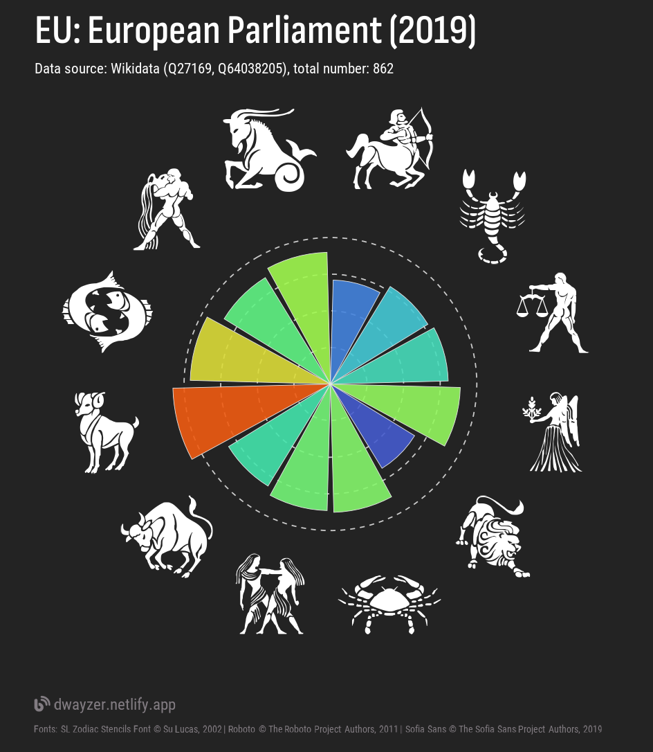

Figure 1: Zodiac portrait of the MEPs elected into 9th EU Parliament

Show code

uk_chart_file <- paste0(dir_charts, "uk_west_zodiac.png")

if(!file.exists(uk_chart_file)){
  title <- "UK: the House of Commons (2019)"
  subtitle <- paste0("Data source: Wikidata (Q77685926), total number: ", 
                     scales::number(nrow(us), big.mark = ","))
  
  ch <- west_zodiac_chart(df = uk, 
                          symbols_table = west_symbols, 
                          ch_title = title,
                          ch_subtitle = subtitle)
  
  ggplot2::ggsave(filename = uk_chart_file, plot = ch, 
                  height = 9.2, width = 8, units = "cm", dpi = 300)
}
knitr::include_graphics(uk_chart_file)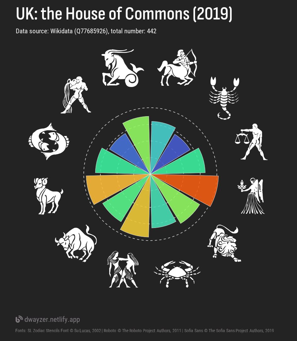

Figure 2: Zodiac portrait of the MPs elected into UK Parliament in 2019

Show code

us_chart_file <- paste0(dir_charts, "us_west_zodiac.png")

if(!file.exists(us_chart_file)){
  title <- "US: the House of Representatives (2019)"
  subtitle <- paste0("Data source: Wikidata (Q13218630, Q65089999), total number: ", 
                     scales::number(nrow(us), big.mark = ","))
  
  ch <- west_zodiac_chart(df = us, 
                          symbols_table = west_symbols, 
                          ch_title = title, 
                          ch_subtitle = subtitle)
  
  ggplot2::ggsave(filename = us_chart_file, plot = ch, 
                  height = 9.2, width = 8, units = "cm", dpi = 300)
  
  remove(ch, title, subtitle)
}
knitr::include_graphics(us_chart_file)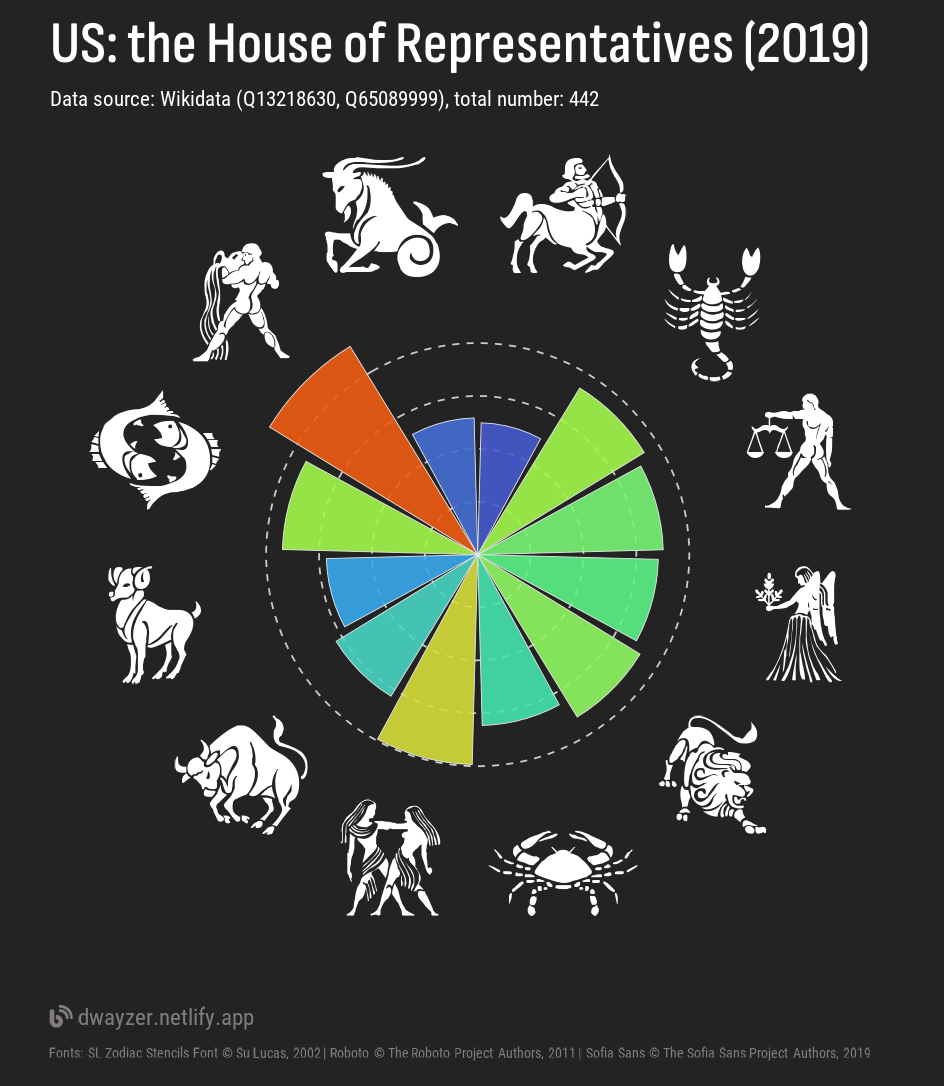

Figure 3: Zodiac portrait of the politicians elected into the US House of Representatives (the 117th US Congress)

Show code

fr_chart_file <- paste0(dir_charts, "fr_west_zodiac.png")

if(!file.exists(fr_chart_file)){
  title <- "FR: the 16th legislature (2022)"
  subtitle <- paste0("Data source: Wikidata (Q3044918, Q112567597), total number: ", 
                     scales::number(nrow(fr), big.mark = ","))
  
  ch <- west_zodiac_chart(df = fr, 
                          symbols_table = west_symbols, 
                          ch_title = title, 
                          ch_subtitle = subtitle)
  
  ggplot2::ggsave(filename = fr_chart_file, plot = ch, 
                  height = 9.2, width = 8, units = "cm", dpi = 300)
  
  remove(ch, title, subtitle)
}
knitr::include_graphics(fr_chart_file)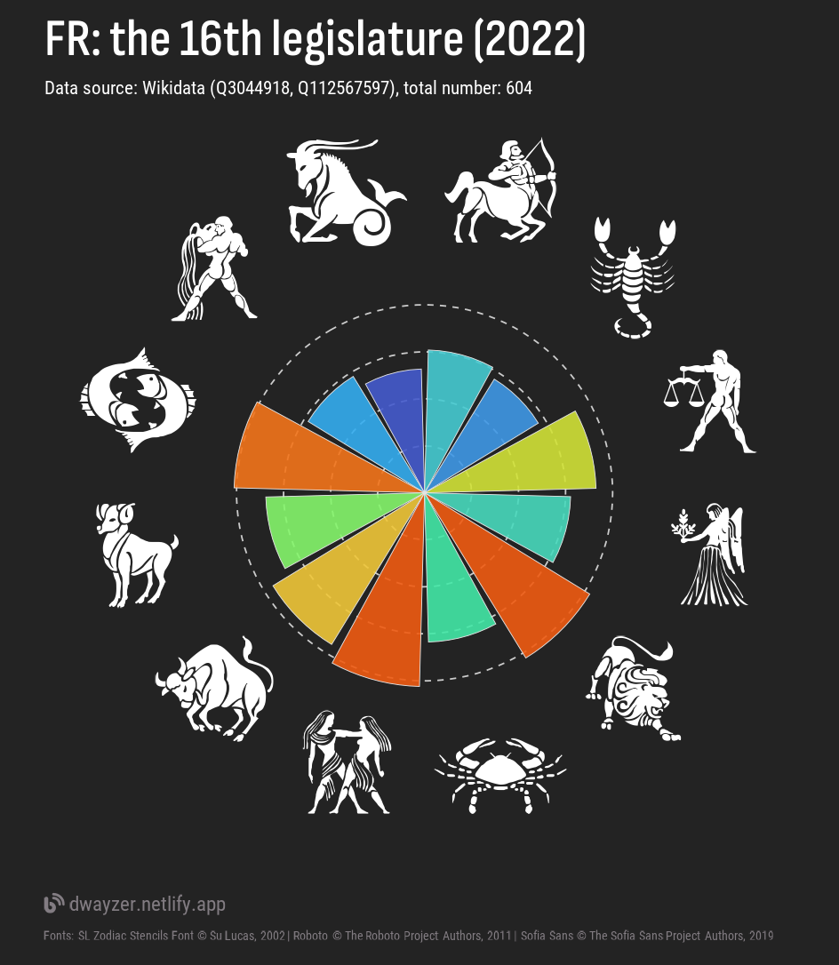

Figure 4: Zodiac portrait of the politicians elected into the 16th legislature of the 5th French Republic (French National Assembly) (2021)

Show code

de_chart_file <- paste0(dir_charts, "de_west_zodiac.png")

if(!file.exists(de_chart_file)){
  title <- "DE: the 20th German Bundestag (2021)"
  subtitle <- paste0("Data source: Wikidata (Q1939555, Q33091469), total number: ", 
                     scales::number(nrow(de), big.mark = ","))
  
  ch <- west_zodiac_chart(df = de, 
                          symbols_table = west_symbols, 
                          ch_title = title, 
                          ch_subtitle = subtitle)
  
  ggplot2::ggsave(filename = de_chart_file, plot = ch, 
                  height = 9.2, width = 8, units = "cm", dpi = 300)
  
  remove(ch, title, subtitle)
}
knitr::include_graphics(de_chart_file)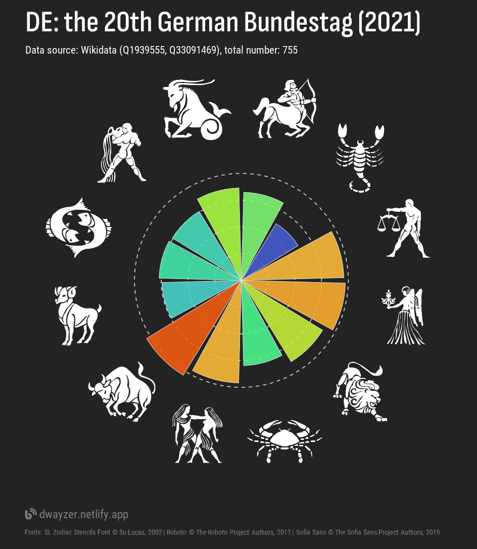

Figure 5: Zodiac portrait of the politicians elected into the 20th German Bundestag (2021)

Show code

ru_chart_file <- paste0(dir_charts, "ru_west_zodiac.png")

if(!file.exists(ru_chart_file)){
  title <- "RU: the 8th Russian Duma (2021)"
  subtitle <- paste0("Data source: Wikidata (Q17276321, Q106638694), total number: ", 
                     scales::number(nrow(ru), big.mark = ","))
  
  ch <- west_zodiac_chart(df = ru, 
                          symbols_table = west_symbols, 
                          ch_title = title, 
                          ch_subtitle = subtitle)
  
  ggplot2::ggsave(filename = ru_chart_file, plot = ch, 
                  height = 9.2, width = 8, units = "cm", dpi = 300)
  
  remove(ch, title, subtitle)
}
knitr::include_graphics(ru_chart_file)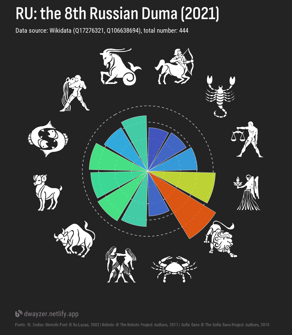

Figure 6: Zodiac portrait of the members of the VIII’s Russian State Duma (2021)

Chinese Zodiac Chart

Here is another function that draws a chart for Chinese zodiac signs, with the following arguments:

df (a dataframe from Wikidata with dob column)
ch_dates (the date range for the Chinese calendar years. In this script it is named “ch_dates”). I also use a function get_ch_sign() to find a chinese zodac year for a specified date.
symbols_table (a table that orders the zodiac signs and link them to font-coding letters. In this script it is named “east_symbols”)
title
subtitle

Show code

# converting the chinese dates into integer
ch_dates <- ch_dates |>
  mutate(across(contains("date"), ~as.integer(.x), .names = "{.col}_int"))

# function to assign the chinese zodiac signs 
get_ch_sign <- function(date, ch_dates){
  date <- as.integer(as.Date(date))
  k <- ch_dates |> filter(date_start_int <= date & date_end_int >= date)
  if(nrow(k)>1 | nrow(k) == 0) { return(NA) } else { return( pull(k, sign) ) }
}

east_zodiac_chart <- function(df, ch_dates, symbols_table, ch_title, ch_subtitle){
  df |>
    mutate(sign = purrr::map_chr(dob, ~get_ch_sign(date = .x, ch_dates)), 
           total = n()) |>
    count(total, sign) |>
    left_join(symbols_table, by = join_by(sign)) |> 
    arrange(order) |> na.omit() |> 
    mutate(n = 2000*n/total) |>
    ggplot() +
    geom_hline(yintercept = base::pretty(c(0,200), n = 5),
               linetype = 2, linewidth = 0.2, colour = "grey80") +
    geom_col(aes(x = order, y = n*1.02, fill = n), 
             alpha = 0.9, width = 0.9, colour = "grey90", linewidth = 0.1) +
    geom_richtext(aes(x = order, y = 315, label = letter),
                      vjust = 0.48, hjust = 0.48, colour = "white", family = "ch_zodiac", 
                      size = 18, label.colour = NA, fill = NA)+
    scale_x_reverse(expand = expansion(add = 0.05))+
    coord_polar(start = -pi / 6) +
    scale_fill_viridis_c(option = "H", direction = 1, begin = 0.1, end = 0.8)+
    guides(fill = "none") + 
    blankbg +
    labs(title = ch_title, 
         subtitle = ch_subtitle, 
         caption = paste0("<span style='font-family:\"fa_solid\"'>&#xf781;</span>",
                         "<span style='font-family:\"RobotoC\";'>   dwayzer.netlify.app</span>",
                         "<br/><span style='font-family:\"RobotoC\"; font-size:\"5.3pt\";'>",
                         "Fonts: Chinese Zodiac | ",
                         "Roboto &#169; The Roboto Project Authors, 2011 | ",
                         "Sofia Sans &#169; The Sofia Sans Project Authors, 2019</span>"))
}

Show code

eu_chart_file <- paste0(dir_charts, "eu_east_zodiac.png")

if(!file.exists(eu_chart_file)){
  title <- "EU: European Parliament (2019)"
  subtitle <- paste0("Data source: Wikidata (Q27169, Q64038205), total number: ", 
                     scales::number(nrow(eu), big.mark = ","))
  
  ch <- east_zodiac_chart(df = eu, 
                          ch_dates = ch_dates,
                          symbols_table = east_symbols, 
                          ch_title = title,
                          ch_subtitle = subtitle)
  
  ggplot2::ggsave(filename = eu_chart_file, plot = ch, 
                  height = 9.2, width = 8, units = "cm", dpi = 300)
}
knitr::include_graphics(eu_chart_file)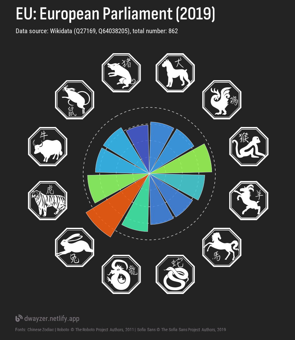

Figure 7: Chinese zodiac portrait of the MEPs elected into 9th EU Parliament

Show code

uk_chart_file <- paste0(dir_charts, "uk_east_zodiac.png")

if(!file.exists(uk_chart_file)){
  title <- "UK: the House of Commons (2019)"
  subtitle <- paste0("Data source: Wikidata (Q77685926), total number: ", 
                     scales::number(nrow(us), big.mark = ","))
  
  ch <- east_zodiac_chart(df = uk, 
                          ch_dates = ch_dates,
                          symbols_table = east_symbols, 
                          ch_title = title,
                          ch_subtitle = subtitle)
  
  ggplot2::ggsave(filename = uk_chart_file, plot = ch, 
                  height = 9.2, width = 8, units = "cm", dpi = 300)
}
knitr::include_graphics(uk_chart_file)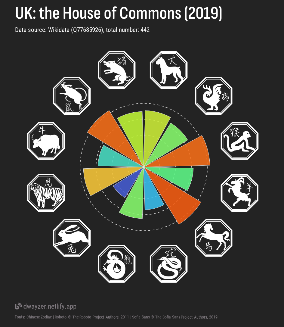

Figure 8: Chinese zodiac portrait of the MPs elected into UK Parliament in 2019

Show code

us_chart_file <- paste0(dir_charts, "us_east_zodiac.png")

if(!file.exists(us_chart_file)){
  title <- "US: the House of Representatives (2019)"
  subtitle <- paste0("Data source: Wikidata (Q13218630, Q65089999), total number: ", 
                     scales::number(nrow(us), big.mark = ","))
  
  ch <- east_zodiac_chart(df = us, 
                          ch_dates = ch_dates,
                          symbols_table = east_symbols, 
                          ch_title = title, 
                          ch_subtitle = subtitle)
  
  ggplot2::ggsave(filename = us_chart_file, plot = ch, 
                  height = 9.2, width = 8, units = "cm", dpi = 300)
  
  remove(ch, title, subtitle)
}
knitr::include_graphics(us_chart_file)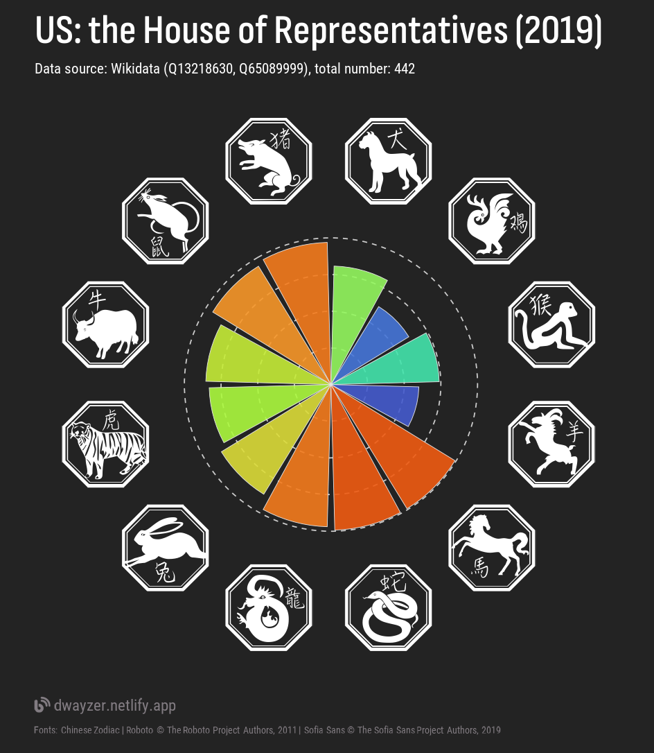

Figure 9: Chinese zodiac portrait of the politicians elected into the US House of Representatives (the 117th US Congress)

Show code

fr_chart_file <- paste0(dir_charts, "fr_east_zodiac.png")

if(!file.exists(fr_chart_file)){
  title <- "FR: the 16th legislature (2022)"
  subtitle <- paste0("Data source: Wikidata (Q3044918, Q112567597), total number: ", 
                     scales::number(nrow(fr), big.mark = ","))
  
  ch <- east_zodiac_chart(df = fr, 
                          ch_dates = ch_dates,
                          symbols_table = east_symbols, 
                          ch_title = title, 
                          ch_subtitle = subtitle)
  
  ggplot2::ggsave(filename = fr_chart_file, plot = ch, 
                  height = 9.2, width = 8, units = "cm", dpi = 300)
  
  remove(ch, title, subtitle)
}
knitr::include_graphics(fr_chart_file)

Chinese zodiac portrait of the politicians elected into the 16th legislature of the 5th French Republic (French National Assembly) (2021)

Figure 10: Chinese zodiac portrait of the politicians elected into the 16th legislature of the 5th French Republic (French National Assembly) (2021)

Show code

de_chart_file <- paste0(dir_charts, "de_east_zodiac.png")

if(!file.exists(de_chart_file)){
  title <- "DE: the 20th German Bundestag (2021)"
  subtitle <- paste0("Data source: Wikidata (Q1939555, Q33091469), total number: ", 
                     scales::number(nrow(de), big.mark = ","))
  
  ch <- east_zodiac_chart(df = de, 
                          ch_dates = ch_dates,
                          symbols_table = east_symbols, 
                          ch_title = title, 
                          ch_subtitle = subtitle)
  
  ggplot2::ggsave(filename = de_chart_file, plot = ch, 
                  height = 9.2, width = 8, units = "cm", dpi = 300)
  
  remove(ch, title, subtitle)
}
knitr::include_graphics(de_chart_file)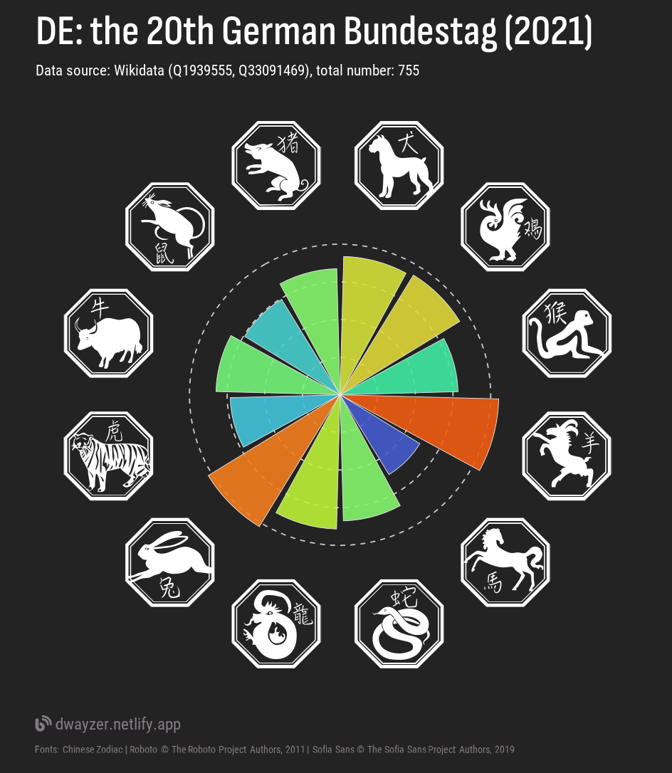

Figure 11: Chinese zodiac portrait of the politicians elected into the 20th German Bundestag (2021)

Show code

ru_chart_file <- paste0(dir_charts, "ru_east_zodiac.png")

if(!file.exists(ru_chart_file)){
  title <- "RU: the 8th Russian Duma (2021)"
  subtitle <- paste0("Data source: Wikidata (Q17276321, Q106638694), total number: ", 
                     scales::number(nrow(ru), big.mark = ","))
  
  ch <- east_zodiac_chart(df = ru, 
                          ch_dates = ch_dates,
                          symbols_table = east_symbols, 
                          ch_title = title, 
                          ch_subtitle = subtitle)
  
  ggplot2::ggsave(filename = ru_chart_file, plot = ch, 
                  height = 9.2, width = 8, units = "cm", dpi = 300)
  
  remove(ch, title, subtitle)
}
knitr::include_graphics(ru_chart_file)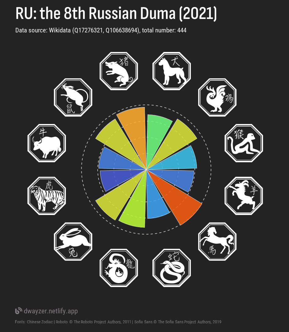

Figure 12: Chinese zodiac portrait of the members of the VIII’s Russian State Duma (2021)

Combo Charts

In a chunk below I build a preview chart for this post. For that purpose I am using a patchwork package.

Show code

eu_chart_file <- paste0(dir_charts, "eu_combo_zodiac.png")

if(!file.exists(eu_chart_file)){
  library(patchwork)
  ch1 <- west_zodiac_chart(df = eu, symbols_table = west_symbols, 
                          ch_title = NULL, ch_subtitle = NULL) + 
    labs(caption = NULL)
  ch2 <- east_zodiac_chart(df = eu, ch_dates, symbols_table = east_symbols, 
                          ch_title = NULL, ch_subtitle = NULL) + 
    labs(caption = NULL)
  
 ch <- (free(ch1) + free(ch2)) + 
   plot_annotation(
     title = 'Zodiac Charts for the 9th European Parliament MEPs',
     subtitle = paste0("Data source: Wikidata. Query: SELECT DISTINCT ?item ?dob WHERE {?item p:P39 ?pSt. ?pSt ps:P39 wd:Q27169; pq:P2937 wd:Q64038205. ?item wdt:P569 ?dob.}"),
    caption = paste0("<span style='font-family:\"fa_solid\"'>&#xf781;</span>",
                        "<span style='font-family:\"RobotoC\";'>   dwayzer.netlify.app</span>",
                        "<br/><span style='font-family:\"RobotoC\"; font-size:\"7.3pt\";'>",
                        "Fonts: SL Zodiac Stencils Font &#169; Su Lucas, 2002 | Chinese Zodiac | ",
                        "Roboto &#169; The Roboto Project Authors, 2011 | ",
                        "Sofia Sans &#169; The Sofia Sans Project Authors, 2019</span>"),
    theme = blankbg + theme(plot.caption = element_markdown(hjust = 1, halign = 1))) &
   theme(plot.margin = unit(c(t=0.2,r=0.1,b=0.2,l=0.1), "cm"))
   
   
  ggplot2::ggsave(filename = eu_chart_file, plot = ch, 
                  height = 9, width = 14, units = "cm", dpi = 300)
}
knitr::include_graphics(eu_chart_file)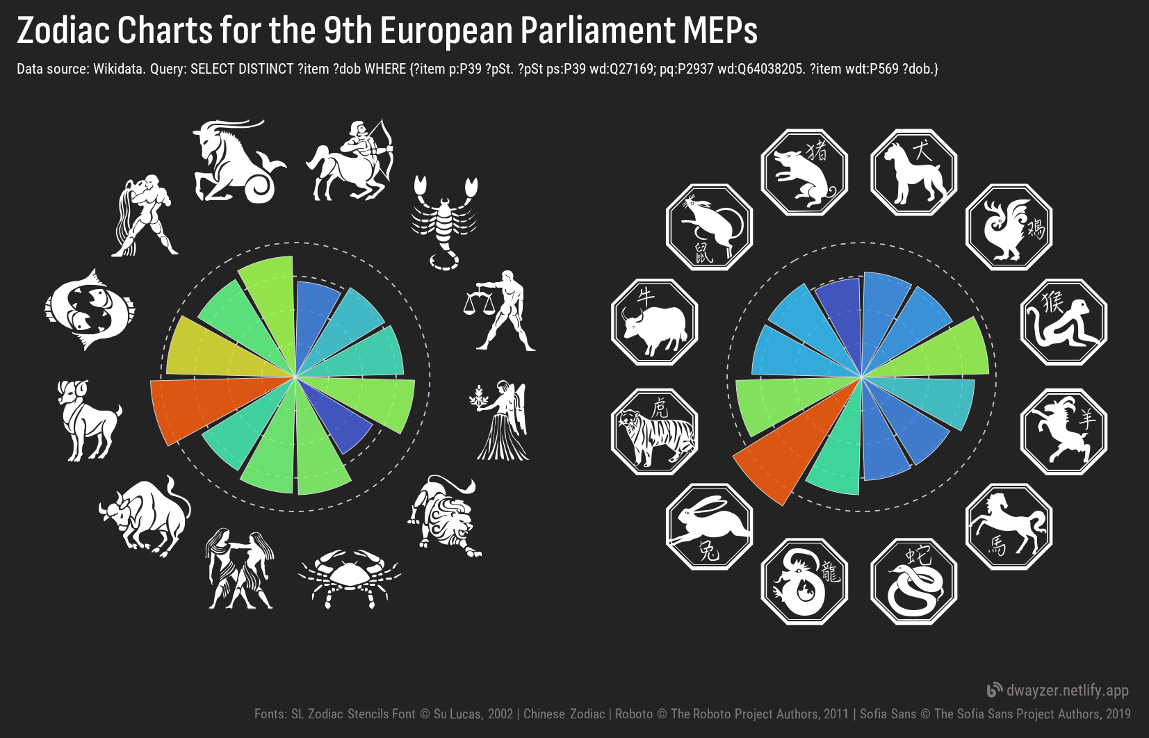

Things I would do…

…if I had a spare time, of course. Even though we see that the national parliaments have some peculiar differences, it would be much more interesting to see how different are the left- and right- political parties. Of course, one may argue that for many politicians a party is not a choice dictated by temper or morality, but rather a career-wise opportunity the person decided to take and pursue at some moment of life. Alas, this could be true.

Another interesting exercise would be to make a metric to assess an astrological stability of the groups and committees, with a special attention to those formed not via independent voting, but through the appointments (i.e. the members are picked up or recommended by a team leader, or senior members).

Acknowledgments

Allaire J, Xie Y, Dervieux C, McPherson J, Luraschi J, Ushey K, Atkins A, Wickham H, Cheng J, Chang W, Iannone R (2023). rmarkdown: Dynamic Documents for R. R package version 2.22, https://github.com/rstudio/rmarkdown.

Pedersen T (2024). patchwork: The Composer of Plots. R package version 1.2.0, https://CRAN.R-project.org/package=patchwork.

Popov M (2020). WikidataQueryServiceR: API Client Library for ‘Wikidata Query Service’. R package version 1.0.0, https://CRAN.R-project.org/package=WikidataQueryServiceR.

Qiu Y, details. aotifSfAf (2022). sysfonts: Loading Fonts into R. R package version 0.8.8, https://CRAN.R-project.org/package=sysfonts.

Qiu Y, details. aotisSfAf (2023). showtext: Using Fonts More Easily in R Graphs. R package version 0.9-6, https://CRAN.R-project.org/package=showtext.

Wickham H (2022). stringr: Simple, Consistent Wrappers for Common String Operations. R package version 1.5.0, https://CRAN.R-project.org/package=stringr.

Wickham H (2016). ggplot2: Elegant Graphics for Data Analysis. Springer-Verlag New York. ISBN 978-3-319-24277-4, https://ggplot2.tidyverse.org.

Wickham H, François R, Henry L, Müller K, Vaughan D (2023). dplyr: A Grammar of Data Manipulation. R package version 1.1.2, https://CRAN.R-project.org/package=dplyr.

Wickham H, Henry L (2023). purrr: Functional Programming Tools. R package version 1.0.1, https://CRAN.R-project.org/package=purrr.

Wickham H, Hester J, Bryan J (2023). readr: Read Rectangular Text Data. R package version 2.1.4, https://CRAN.R-project.org/package=readr.

Wickham H, Seidel D (2022). scales: Scale Functions for Visualization. R package version 1.2.1, https://CRAN.R-project.org/package=scales.

Wickham H, Vaughan D, Girlich M (2023). tidyr: Tidy Messy Data. R package version 1.3.0, https://CRAN.R-project.org/package=tidyr.

Wilke C, Wiernik B (2022). ggtext: Improved Text Rendering Support for ‘ggplot2’. R package version 0.1.2, https://CRAN.R-project.org/package=ggtext.

Xie Y (2023). knitr: A General-Purpose Package for Dynamic Report Generation in R. R package version 1.43, https://yihui.org/knitr/.

Xie Y (2015). Dynamic Documents with R and knitr, 2nd edition. Chapman and Hall/CRC, Boca Raton, Florida. ISBN 978-1498716963, https://yihui.org/knitr/.

Xie Y (2014). “knitr: A Comprehensive Tool for Reproducible Research in R.” In Stodden V, Leisch F, Peng RD (eds.), Implementing Reproducible Computational Research. Chapman and Hall/CRC. ISBN 978-1466561595.

Xie Y, Allaire J, Grolemund G (2018). R Markdown: The Definitive Guide. Chapman and Hall/CRC, Boca Raton, Florida. ISBN 9781138359338, https://bookdown.org/yihui/rmarkdown.

Xie Y, Dervieux C, Riederer E (2020). R Markdown Cookbook. Chapman and Hall/CRC, Boca Raton, Florida. ISBN 9780367563837, https://bookdown.org/yihui/rmarkdown-cookbook.

Zodiac Charts

Notes on Code

Fonts

Extra Data

Data

Western Zodiac Chart

Chinese Zodiac Chart

Combo Charts

Things I would do…

Acknowledgments

Reuse

Citation